TAX RATES AND THE U.S. ECONOMY
Introduction
Most, if not all, Republicans believe that lower federal tax rates will cause the economy to improve. Indeed, sometimes it seems as if they have no other economic policy and their answer to any problem in the economy is tax reduction. Usually the conversation is about personal income tax, but various Republicans and conservative commentators also recommend lowering capital gains tax rates or corporate income tax rates or both. Some Democrats occasionally join them in such recommendations. The reasoning generally is along the lines that if the tax-paying public has more after-tax income, they will spend it in a manner that stimulates the economy, a perfectly reasonable theory.
I wish to make clear at the start that this study is not about any economic theory, reasonable or not. What follows is an empirical study of what has occurred in the past 65 years (1950 through 2014) of U.S. history. It is simply history and math; I am not concerned with whether the discoveries conform to any theory and offer none to explain the results.
Two measures of the economy are used herein: GDP (gross domestic product) growth rate and job growth rate. Linear regression of these measures over the period is performed with each of three federal tax rates: top marginal personal income tax, top marginal corporate income tax, and top marginal long-term capital gains tax. Then multiple linear regression of each of the two economic measures with all three tax rates is also considered. Linear regression calculations tell us to what extent the variables are correlated and also how much of the variation in the economic measures is possibly linearly attributable to changes in the tax rates.
All data represent annual averages. The starting year, 1950, was chosen to be as early as possible while avoiding the distortion of the economy by World War II. Also I am unsure of the reliability of earlier figures and they are more difficult to find. The ending year, 2014, is the latest for which complete figures are available at the time of this writing. Thus I tried to be as inclusive as possible. The calculation software is Origin® 2015. The data sources used are
· GDP growth rate – U.S. Bureau of Economic Analysis, www.bea.gov
· Job growth rate – U.S. Bureau of Labor Statistics, www.bls.gov
· Personal income tax rates – U.S. Internal Revenue Service, www.irs.gov, or the Tax Foundation, www.taxfoundation.org
· Corporate income tax – Tax Policy Center, www.taxpolicycenter.org
· Long-term capital gains tax – U.S. Internal Revenue Service, www.irs.gov, or the Tax Policy Center, www.taxpolicycenter.org
Note on the Independent Variables
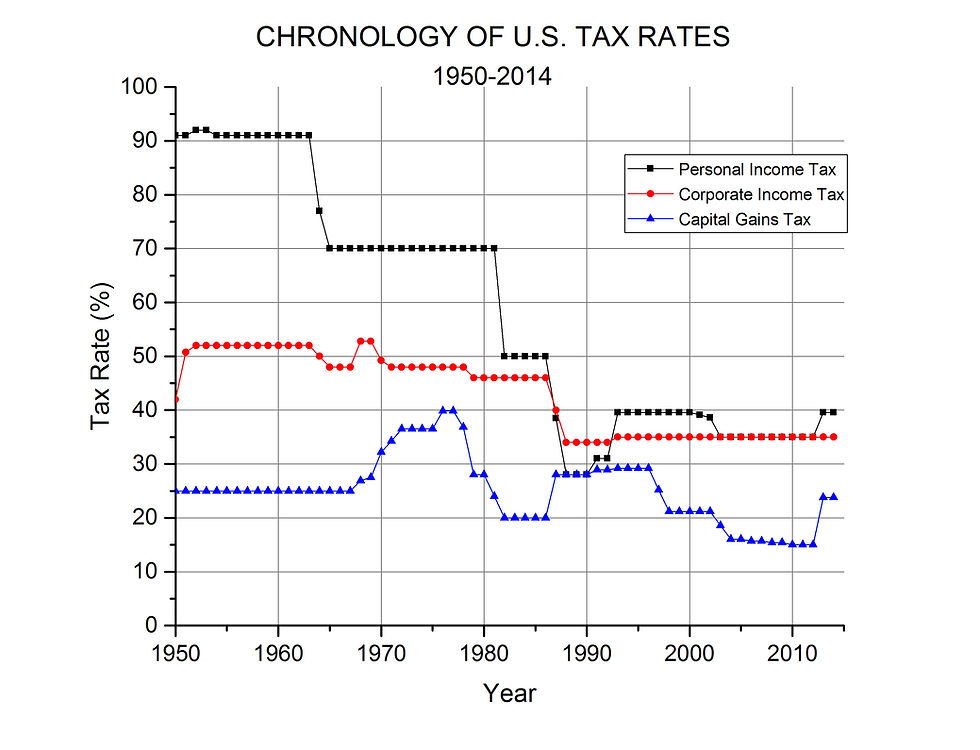
The three tax rates are considered independent variables because they may be set arbitrarily by the federal government. All three rates, despite some ups and downs, have generally declined over the 65 year period: they are lower in 2014 than it 1950. Figure 1 shows the history.
FIGURE 1

For the last two years the top marginal long-term capital gains tax rate has come back to nearly where it was in 1950, although it was lower than that for more than the previous decade.
Of course there have been other changes in federal tax law that could affect the health of the economy. Changes in the number of tax brackets, the upper and lower bounds of the brackets, allowed deductions, length of time of ownership for an asset to qualify as “long-term”, to name a few. These are more difficult to quantify and are not considered in this study.
Personal Income Tax
The personal income tax rate is the one that receives the most political attention. It is also the one that has varied the most, from 92% in 1952-1953 to 28% in 1988-1990. Because of the large variation over the years, one would expect this rate to have had the most effect on the economic measures. Figure 2 shows the scatterplot between this tax rate and the GDP growth rate.
FIGURE 2
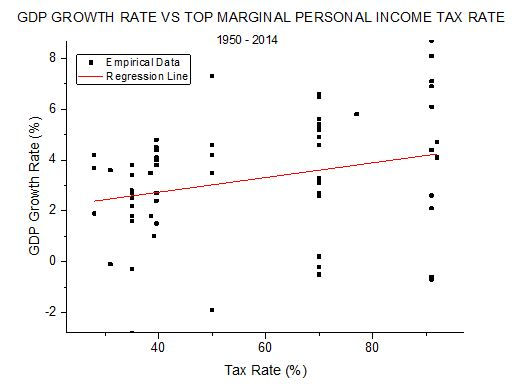
The regression line is the best straight line fit to the data. It has the form

The intercept, a, and the slope, b, are calculated to minimize the mean square error. The results in this case are a = 1.58±.80 and b = 0.03±.01. Even though it is quite small, this slope is considered statistically significant at the 0.05 level. The correlation coefficient between the two variables is r = 0.27 and the coefficient of determination (COD) is r2 = 0.075. This last quantity describes how much of the variation in GDP growth rate could be linearly attributable to variations in the tax rate. The value calculated means that just 7.5% of the variation in GDP growth rate could have possibly come from the changes in personal income tax rate; 92.5% of the variation must have come from other factors. Furthermore, the slope and the correlation are positive which means that if the tax rate has affected the growth rate at all, it has been in the direction of higher taxes causing higher growth. The small correlation and COD values are to be expected when the scatterplot shows the data points scattered far from the regression line. A Congressional Research Service study of 2012 also finds a positive, but statistically insignificant, slope between GDP/capita growth rate and the top marginal personal income tax rate using the same linear regression methods[1].
Next we consider the effect of this tax on job growth. Figure 3 shows the applicable scatterplot.
FIGURE 3
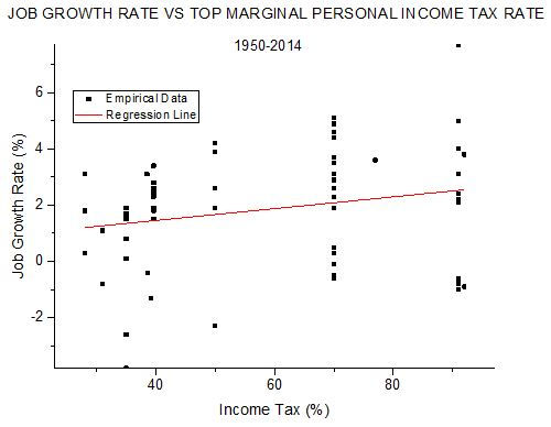
Again the slope and correlation are positive, but smaller than in the case above, and not considered statistically significant. For the sake of completeness, a = 0.62±0.72 and b = 0.021±0.011. Here r = 0.22 and COD = 0.05. Basically, this regression analysis indicates that the job growth rate over the last 65 years shows almost no dependence on the personal income tax rate.
Certainly the numbers show no support at all for the hypothesis that reducing the top marginal personal income tax rate will improve the economy in terms of either GDP growth or job growth.
Corporate Income Tax
This tax rate has varied from 52.8% in 1968-1969 down to 34% in 1988-1992. Its relation to GDP growth rate is shown in the scatterplot of Figure 4.
FIGURE 4
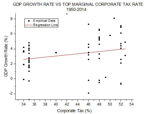
As was the case with personal income tax, the points are very scattered and the regression line slope is positive. With the large scatter and small slope, the latter is not statistically significant. The intercept a = 0.07±1.7 and the slope b = 0.07±0.04; another measure of the large scatter is shown by the uncertainties in these values being as large as, or larger than, the values themselves. In this instance r=0.23 and COD=0.05. These results mean that the corporate income tax seems to have had little effect on GDP growth, possibly accounting for no more than 5% of the variation of the latter. Certainly there is no indication that higher corporate income tax rates adversely affect GDP growth.
Next we look at the effect on job growth. Figure 5 illustrates.
FIGURE 5
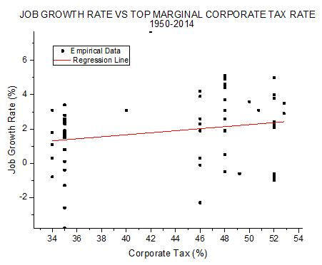
This looks much like Figure 4: much scatter, and a small, statistically insignificant, positive slope. a=-0.70±1.5, b=0.06±0.04, r=0.21, and COD=0.04. This COD value is even smaller than that for GDP growth and means that only 4% of the variation in job growth could be due to corporate income tax rate. Again this result provides no support for the hypothesis that higher tax rates hurt the economy.
Capital Gains Tax
This tax is the most complicated of the three. Not only have the rates changed over the years, but also the brackets, the definition of “long-term”, and various other aspects. For example, some assets like art objects have had their own special rates. I have not taken such special cases into account, only the top marginal rate for the majority of assets. That rate has varied from to 39.875% in 1976-1977 down to 15% in 2010-2012. The scatterplot of Figures 6 and 7 shows the relation of that rate to the two economic measures.
FIGURE 6
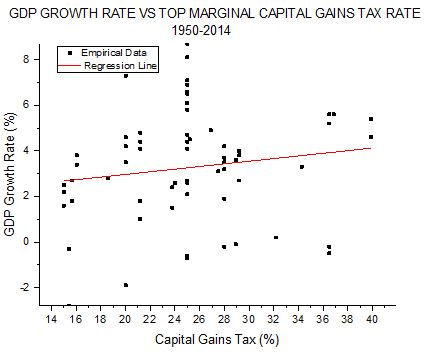
FIGURE 7
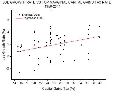
These two plots look monotonously similar to each other and to the four previous scatterplots. They all show regression lines with slight positive slope and a great deal of scatter of the empirical points away from that line. What they do not show is any tendency for higher tax rates to harm the economy. The table below shows the parameters calculated for the dependence of the economic measures on the top marginal long-term capital gains tax rate.

Because of the relatively large correlation coefficient and COD values (corresponding to less scatter), the slope in Figure 7 is considered statistically significant, just as in the case of GDP growth versus personal income tax rate.
Three Tax Rates Considered Together
Although all the calculations up to this point show weak evidence for improvement in the economy with higher tax rates, that could be due to other variables that affect the economy. After all, the largest coefficient of determination found was the last one, CD=0.09, in which case 91% of the variation in the economic measure must be due to variables not considered. Variables not considered in any one of the regression calculations could include the other two tax rates. By performing multiple linear regression for each of the two economic measures using all three tax rates, we at least eliminate that source of confusion. Multiple linear regression means finding a linear equation of the form,

and where the intercept, a, and coefficients, b,c,d, minimize the mean square error given all the data. This equation corresponds to a three-dimensional hyperplane in a four-dimensional scatterplot, analogous to the regression lines displayed above. Unfortunately I cannot draw such a geometrical representation, but I can carry out the calculation.
The following table summarizes the multiple regression results.

The coefficient of determination still tells what fraction of the variation in the dependent variable could be attributed to the variations in the multiple independent variables. In our case we see that 8.4% of the GDP growth variation and 11% of the job growth variation can be so attributed. Another important outcome is that the coefficient of the corporate income tax rate has turned negative, the first hint that raising a tax rate could lower growth rates. This evidence is very weak because the magnitude of the uncertainty in that coefficient is nearly 20 times greater than the coefficient in one case, and 3 times greater in the other. The numbers (positive coefficients) still indicate that raising either, or both, of the other two tax rates would raise the growth rates.
Population
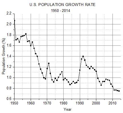
There is one independent variable that might well have an effect on economic growth and that is population growth. Generally, the larger the population of a country, the larger the GDP. It is difficult to see how population growth in any year can fail to increase GDP because every additional resident, even newborns and illegal immigrants, creates additional demand for goods and services. Population growth rate over the period[2] is shown in Figure 8. It can be seen that this variable has generally declined over the period like the tax rates, so some of the variation we see in economic growth rates could be due to this variable rather than the taxes. The only way to tell is to include this variable with taxes in multiple linear regression. Of course, population growth rate is not a variable directly controllable by the government.
FIGURE 8
The results of the multiple linear regression are shown in the table below.

When the values in this table are compared to those in the previous table, we see that adding the population growth rate into the analysis has a significant effect on the tax coefficients for GDP growth, but very little effect on the coefficients for job growth. For GDP growth, population growth becomes the major factor because it has the largest coefficient. Furthermore, all the coefficients are now positive and the COD value has increased significantly. The positive signs mean that increasing any of the tax rates (or the population growth rate) leads to an increase in GDP growth. For job growth, the tax rate coefficients change little, the coefficient for corporate tax is still negative, the COD value changes only in the fourth decimal place, and the coefficient for population growth is not the largest one. Basically, these new coefficients tell us how economic growth would depend on tax rates if population growth were zero
Conclusions
The most robust finding of this study is that the tax rates have had little to no effect on the economy. Even if we assume that there is a causal relationship between the three tax rates and economic growth, all three rates together can account for no more than 8.4% of the variation in the GDP growth rate and 11% of the variation in the job growth rate. These percentages represent a maximum in a linear relationship; the tax rate effect could be less but not more.
If we do accept the causal assumption then we are forced to accept that it is likely that both the personal income tax rate and the capital gains tax rate cause better economic growth when they are higher (positive coefficients in the multiple linear regression equation). There is weak evidence that the corporate income tax rate works in accord with conventional wisdom in the case of job growth, but not GDP growth; the evidence is its negative multiple linear regression coefficient but the weakness comes from the magnitude of the standard error being much larger than the magnitude of the coefficient.
I add one final note. People who believe that lower tax rates are an economic panacea can, and often do, find and trumpet a small subset of the data I used that supports their position. Such a procedure represents a classic case of confirmation bias: promulgating evidence that supports one’s predetermined belief, while ignoring, or even suppressing, evidence that contradicts that belief. I think that I have avoided that error.
Gary Waldman
November 2015
[1] Thomas L. Hungerford, Taxes and the Economy: An Economic Analysis of the Top Tax Rates Since 1945, Sept. 2012, Congressional Research Service Report 7-5700
[2] www.multpl.com/us-population-growth-rate/table/by-year
HIGHER FEDERAL TAXES DO NOT IMPEDE ECONOMIC GROWTH
Introduction
In 2015 I produced a study[1] that definitively showed that higher top marginal individual income tax rates and top marginal corporate income tax rates do not cause lower GDP growth rates. In that work I simply carried out linear regression analyses between the annual GDP growth rate and those tax rates for the years 1950 through 2014. The results showed a positive slope, or positive correlation in both cases: higher economic growth accompanied higher tax rates for the 65 year period.
That study did not prove that higher federal taxes in general do not harm economic growth, because the great majority of people never pay taxes at those rates. Even rich taxpayers whose income reaches the threshold for the top marginal rate do not, on average, pay taxes at that rate on all their income. It can be argued that such a small percentage of aggregate U.S income is taxed at the top rates, it is no wonder that top marginal rates have little effect on the economy.
A better measure of federal tax burden for the tax-paying public as a whole would be some average tax rate. As of June 2016, the Congressional Budget Office has published a table of average household tax rates by income quintiles[2], as well as for all quintiles together (basically all reporting households), for the 81st to 90th percentiles, the 91st to 95th percentiles, the 96th to 99th percentiles, and the top 1%, for the years 1979-2013. These tax rates are calculated straightforwardly by dividing taxes paid by comprehensive income. They include the whole federal tax burden of individual income tax, payroll taxes, corporate income taxes and excise taxes. Individual income taxes are attributed directly to households paying those taxes. Social insurance, or payroll, taxes are attributed to households paying those taxes directly or paying them indirectly through their employers. Corporate income taxes are attributed to households according to their share of capital income. Federal excise taxes are attributed to them according to their consumption of the taxed good or service. Comprehensive income is explained in the footnotes to the tables, but includes retirement and in-kind benefits (Medicaid, Medicare, food stamps, etc.).
In reference 1 I considered the top marginal, long-term, capital gains tax rate separately, but reference 2 evidently considers that tax as part of income tax, the way it is reported.
Although I prefer using longer time periods than the 35 years covered by these tables, one could find no better measure of the federal tax burden on the U.S. public. Therefore I have used these table values in a linear regression analysis with GDP growth rates to examine the effect of federal tax rates on economic growth.
Taxed Enough Already?
Tea Party demonstrators have railed against taxes and have displayed signs that explained the “TEA” of “Tea Party” as an acronym for “Taxed Enough Already.” The tables of reference 2 give average tax rates for each of the federal taxes and the total of federal taxes. Figure 1 shows the total average federal tax rates for each quintile and for all quintiles together over the period.
Figure 1
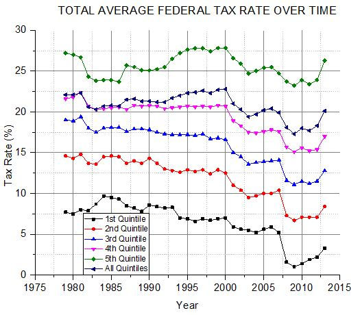
As can be seen, the trend in rates has been generally downward, with every quintile (and all quintiles together) having a lower average rate in 2013 than in 1979. The least change has been for the fifth, or top, quintile: in 1979 the rate was 27.2% and in 2013 it was 26.3%.
I will use the total average federal tax rate values for all quintiles as my measure of tax burden in a linear regression analysis with GDP growth rate for the 35 years.
Taxes – an Impediment to Economic Growth in Theory Only
Figure 2 shows the scatterplot of GDP growth rate[3] versus total average tax rate for all quintiles.
Figure 2

If the federal tax burden were actually an impediment to economic growth, we would expect the slope of the regression line to be negative (lower growth rates accompanying higher tax rates) and the corresponding correlation coefficient to also be negative. Instead both are distinctly positive, statistically significant at the 0.05 level. The correlation coefficient between the two variables is 0.45. The slope of the regression line is 0.6±0.21.
These results make it more likely that higher taxes are a stimulant, rather than an impediment, to economic growth. There are other possible explanations, but here I will just point out that Student’s t-distribution[4] test for statistical significance of a correlation coefficient indicates that the probability of the null result (no real relationship between the variables and the positive correlation just being due to chance) is only 0.325%.
Population
One would think that population growth would be a factor in GDP growth, and so it is in the long-term. Over the 65 year period of 1950 – 2014, there is a statistically significant correlation between annual population growth rate and annual GDP growth rate. The correlation coefficient is 0.277 over that time interval: years with higher population growth generally had higher GDP growth. Reference 1 considers population growth rate along with the top marginal tax rates in a multiple linear regression analysis, and population growth seems to be an important factor.
But that statistical significance is lost in the shorter period 1979 – 2013. For that period the slope of the regression line in a linear regression analysis for GDP growth rate versus population growth rate is not significantly different from zero. That means no discernible relation between the two variables over those 35 years.
Because there is no apparent relationship between population growth and GDP growth over the years 1979 – 2013, we would not expect the population data to add much in a multiple linear regression analysis with total average federal tax rate. Indeed, it doesn’t. But I would note that in such a multiple linear regression calculation, the coefficient of the tax term is still positive (0.83±0.27). Therefore we are justified in concluding that, whether or not population growth is taken into account, higher GDP growth rates tend to accompany higher total average federal tax rates.
Why These Results?
Does a higher tax burden on the public as a whole somehow stimulate economic growth? That is one way to explain the positive correlation, but it is difficult to think of how that could happen. Figure 1 suggests another explanation. All the tax rate curves show a steep drop in 2008 and then a turn back upward in 2011, which suggests to me a connection with the Great Recession and subsequent recovery. Perhaps we are seeing the effect of GDP growth on average total tax rate rather than vice-versa. When GDP growth is high we would expect both individuals and corporations to have more income, which might tend to move the aggregate income of the country into higher tax brackets and cause the total average tax rate to increase. Higher incomes might cause “bracket creep” so to speak. If this is true, there could still be some reciprocal effect of tax rate on GDP, but it is hidden in the results by the effect of GDP on tax rate. Those who religiously believe that higher taxes harm economic growth could argue that the positive correlation (due to GDP effect on taxes) would have been even larger had it not been for this harmful effect.
There is a way to perform a linear regression, correlation analysis between the two variables that admits of causation in only one direction. We may pair the total average federal tax rates of each year with the GDP growth rates of the following year. The former can affect the latter but the latter cannot affect the former. There is some reason to suspect that the average tax rate in one year could affect the GDP growth rate in the following year. Individual income taxes for a given year are not reconciled until after the first quarter of the following year. For households that have underpaid taxes the final payment comes due, and for those who have overpaid, a refund comes sometime after tax returns are filed.
Figure 3 shows the scatterplot for such an analysis. Here tax rate values run over the years 1979-2013 and GDP growth values run over the years 1980-2014.
Figure 3
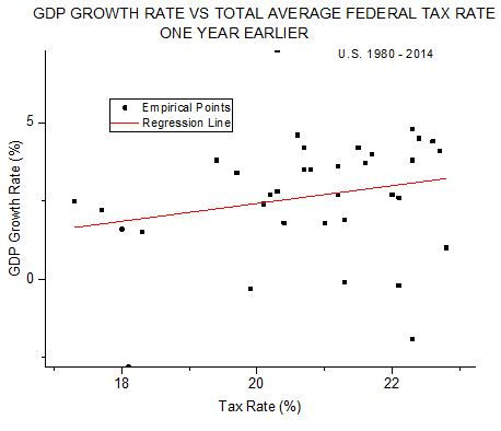
The slope of the regression line is clearly positive, 0.28±0.23, as is the correlation coefficient, 0.21. However, in this case the results are not statistically significant at the 0.05 level. The probability that the null result (no real relationship between the variables) holds is 11.3%. Once again there is not one iota of evidence that higher tax rates impede GDP growth.
Conspiracy of the Uncontrolled Variables
Conservatives who still are determined to cling to their cherished belief that higher taxes hurt the economy have sometimes tried the argument that many other variables affect GDP growth and that the movement of those uncontrolled variables over the 35 years (65 years in the case of reference 1) has magically, not only hidden the “true” effect of taxes on GDP, but also made the opposite correlation appear. I call this hypothesis “the conspiracy of the uncontrolled variables.”
Actually, I have accounted for one other variable, population growth rate, both here and in reference 1, and in neither case does it change the positive correlation between tax rate and GDP growth rate. But, of course, there are many other variables that could be in play. We can be sure this is so, because the index of determination for the analysis of Figure 2, equal to the square of the correlation coefficient, has a value of 0.2. That means that at most 20% of the variation in GDP growth can be due to tax rates (or vice-versa), leaving 80% or more of the variation attributable to other factors.
However, the fact that most of the variation of GDP growth must be due to factors other than tax rates, in no way implies that a “true” relation between that variable and tax rates is likely to be negative. We noted earlier that the probability that, for GDP growth and tax rate of the same year, the “real” result is the null hypothesis, or zero correlation, is a miniscule 0.325%. It is clear that the probability of the correlation and regression line slope “really” being negative is even smaller because a negative correlation is even farther from the calculated value than zero correlation.
A convincing piece of evidence for the hypothesis that higher taxes slow economic growth would be a statistically significant negative correlation. For 35 data points the negative correlation would have to be -0.284 to be statistically significant at the 0.05 level. Once again using Student’s t-statistic, the probability that the “true” correlation is -0.284, when the measured value is 0.45, is only 2.05X10⁻⁷, or 0.00002%.
In the case of the effect of tax rate on GDP growth in the following year, although the measured correlation coefficient is only a statistically insignificant 0.21, the probability of the “true” value being -.284 is only 0.123%. To embrace either of these possibilities is to truly be grasping at straws.
Conclusion
For conservatives, the absolute conviction that higher taxes stifle economic growth is de rigueur. That hypothesis is contradicted by every analysis of empirical data, over 65 years for top marginal rates and over 35 years for total average rates, I have made. The reason conservatives still cling to such a falsehood is more a matter of quasi-religious belief rather than any objective consideration of the facts. The bad news is that, like all religious beliefs, it is impervious to data from the real world. The good news is that the rest of us don’t have to kneel before this shrine of dogma; we can actually look for ourselves and think for ourselves.
Gary Waldman
June 2017
[1] Gary Waldman – TAX RATES AND THE U.S. ECONOMY – November 2015 (available upon request)
[2] www.cbo.gov/publication/51361. Click on “Supplemental Data”. Or see www.taxpolicycenter.org/historical-average-federal-tax-rate-all-households
[3] Growth rates from Bureau of Economic Analysis, www.bea.gov
[4] Sarah Boslaugh – Statistics in a Nutshell – O’Reilly Media Inc., Sebastopol, CA, (2013), pps.186-187
LAFFER, HAUSER, TAX RATES, AND REVENUE
Introduction
Whenever changes in tax rates are discussed, the question of the effect on government revenue arises. At the end of 2015, all Republican candidates for the presidential nomination are advocating tax cuts. All those same candidates, along with all Democrats, would like to reduce the federal deficit. The intuitive feeling is that if tax rates were lower, the government would collect less revenue, increasing the budget deficit. While less revenue for the federal government is just fine with many conservatives, others argue that reducing tax rates would not reduce, and might even increase revenue.
This study seeks to investigate the question of tax rates and government revenue by a statistical analysis of the past 65 years of economic history. The software used for statistical analysis is Origin® 2015. It may not be certain that future economic performance of the national economy will resemble past performance, but I believe strongly that is the way to bet.
The Laffer Curve and “Voodoo Economics”
Many Republicans, and conservatives in general, argue that reducing one or more tax rates would actually bring in more receipts to the federal government, because such reductions would stimulate the economy so much that the additional economic activity would more than compensate for the lower rates. Democrats usually deride this argument as “voodoo economics”, because of its counterintuitive and mysterious nature. However, Democrats were not so derisive in 1963 when the Kennedy administration made essentially the same argument to justify lowering income tax rates. There is nothing inherently irrational in the argument and it should not be dismissed out of hand. Rather, it should be tested against empirical data.
A more detailed, theoretical argument consists of the notorious Laffer Curve. This theory came to prominence during the Reagan administration as a means to justify more tax cuts. Basically, it was noted that government receipts from any tax would be zero for both a 0% rate and a 100% rate, because the former rate is no tax at all and the latter would cause no one to earn, or at least not report any earnings, only to have it all taken by government. It was concluded that a smooth curve must describe government tax receipts versus the tax rate, with a zero at both ends, and a maximum in between. This is the Laffer Curve and a common depiction is shown in Figure 1. Those who want to reduce tax rates usually assume that the rates they wish to reduce are already on the right side of the peak, so lowering the rate would put us farther up the revenue scale. But, of course, there is no way to know just from the theory; I’ve never seen actual numbers on the axes.
FIGURE 1
THE LAFFER CURVE
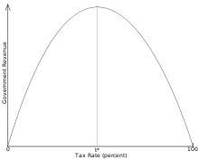
The logic requiring zero revenue at the two extremes, with more revenue generated for tax rates between those, seems unassailable. However, nothing in the logic requires a symmetric curve (as it is always shown), or rules out multiple peaks with valleys in between or a broad plateau in place of a peak. Furthermore it is possible, even likely, that the variations of other economic variables cause the shape of the curve to change annually, or even quarterly.
Perhaps history can give some guidance. The White House Office of Management and Budget gives an historical record[1] of government receipts from individual income tax and corporate income tax separately in nominal dollars. It is a relatively simple matter to convert nominal dollars to constant dollars, in this case 2009 dollars, which removes the effect of inflation. We can then analyze these constant dollar revenues against their respective top, marginal tax rates over the last 65 years of U.S. history. It is possible that we will see a Laffer-type curve, but with actual numbers on the axes, in which case the theory becomes useful. We start with linear regression for receipts vs personal income tax in Figure 2.
FIGURE 2
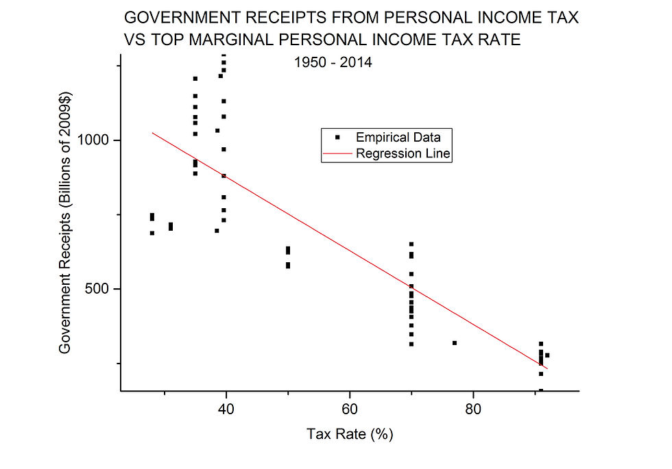
This analysis and graph seem to confirm “voodoo economics” with a vengeance. The slope is significantly different from zero and strongly negative. The coefficient of determination (COD) is 0.75, which means that up to 75% of the variation in government revenue over the years could be explained by just the tax rate: if you want more revenue from personal income taxes, lower the tax rate.
However, something is amiss, because you cannot get ever-increasing revenue from personal income tax by lowering the rate down to zero; the whole idea of the Laffer Curve is that receipts would be zero at 0% tax rate. Somewhere below the historical rates shown, the graph must show a downward trend to the left. Therefore I tried fitting various peak functions to the data of Figure 2. I used the 23 built-in peak functions of Origin® and also a second-order polynomial (which should have a single maximum or minimum). The peak function that fit the best was the Lorentz distribution. I am happy to provide the actual fitting equation to anyone who requests it. The fit gives a COD = 0.84, and is shown below in Figure 3.
FIGURE 3
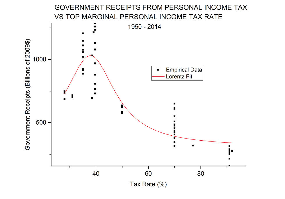
This is a single peak function that actually fits the data better than a straight line and one that could possibly account for up to 84% of the variation in receipts from personal income tax. However it does not go to zero at either end of the tax rate scale, although it does nicely fit data within the historical range of tax rate values.
Moving on to corporate income tax and receipts from that tax, we again start with a simple linear regression, shown in Figure 4. In this case, the slope is significantly different from zero and negative again, but the COD value is only 0.19. None of the peak functions fit very well, and the few that do, look more like an inverted Laffer Curve, because of the low points in the middle of the tax rate range.
FIGURE 4
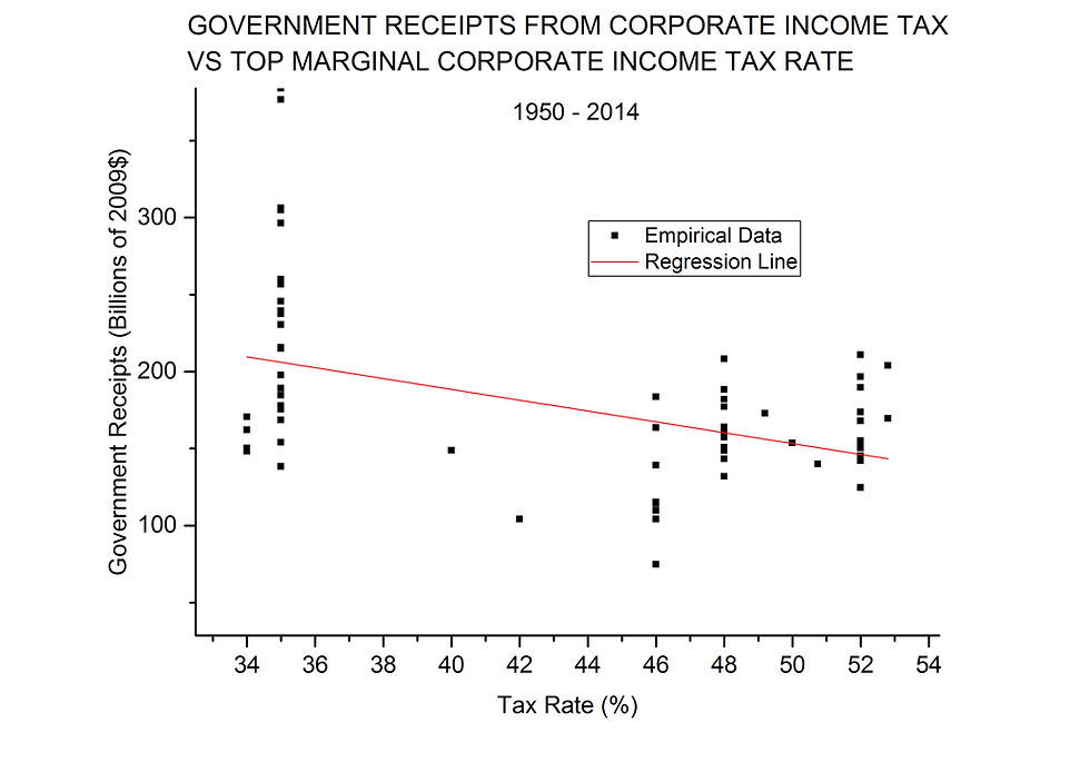
Considering both the personal income tax and the corporate income tax and the revenue they generate, it appears that we have found evidence for “voodoo economics” and, at least in the case of personal income tax, evidence for a Laffer-type curve. But appearances can be deceiving, especially so in this case because we have yet to take into account an important variable. After doing so, we will return to the evidence of Figures 2, 3, and 4.
Gross Domestic Product and Hauser’s Law
We can start by taking an overall view of federal receipts (from all sources) in constant dollars over the whole 65 years. Figure 5 gives a graphic view, with years of personal income tax rate increases marked with blue lines, and years of decreases with red ones. Some of the changes took place in steps over more than one year, but just the first year of change is marked. Data is from the Office of Management and Budget[2].
FIGURE 5
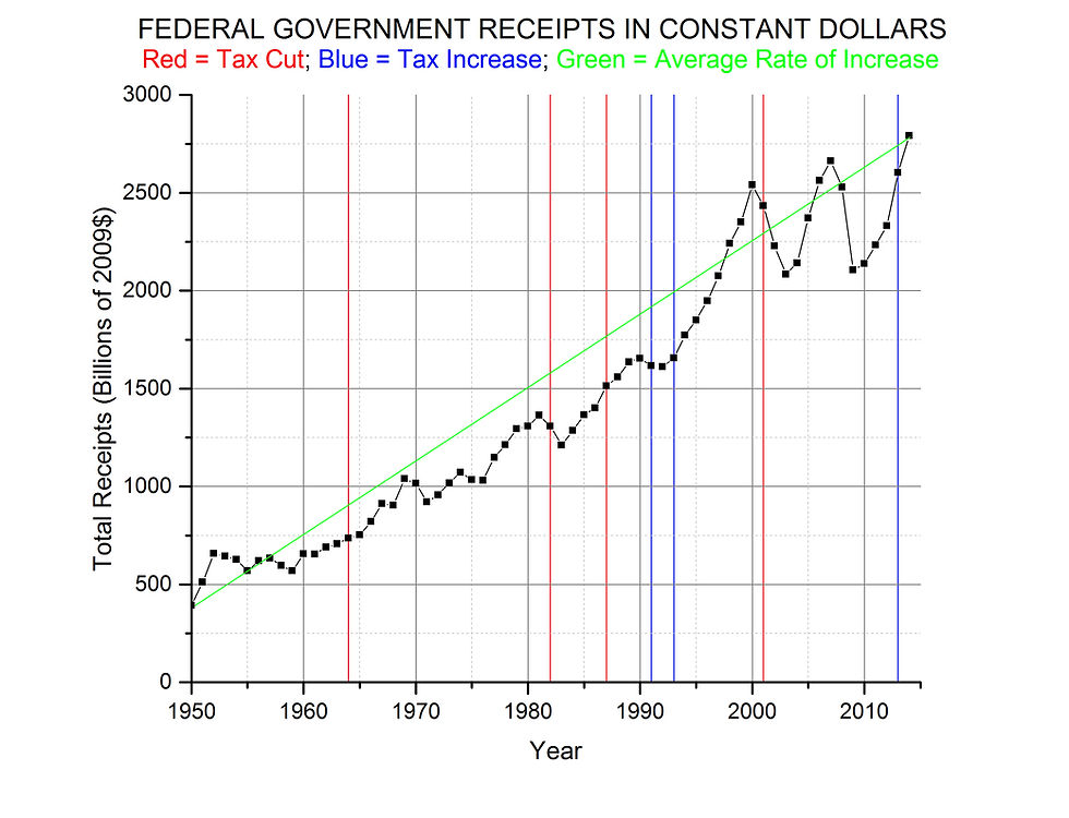
The changes in personal income tax rate seem to have had no consistent effect on total revenue; sometimes they are followed by lower receipts and sometimes higher. Instead, the most striking feature of this overall view is the relentless, almost monotonic rise in government receipts. Remember that inflation has been removed by using constant dollars, so the perceived increase is quite real. Why?
The answer lies in the gross domestic product (GDP) which has also grown in real terms[3] over the same time period, as shown in Figure 6. It is difficult to see how greater GDP could not lead to greater government revenue, regardless of tax rates, because there is more to tax: more personal income, more corporate income, more capital gains, etc.
Additional insight is gained by performing linear regression between total government revenue and GDP. This result is shown in Figure 7. We have a nearly perfect linear fit. COD = 0.97; 97% of the variation in revenue can be explained by just the variable GDP. This fact leads to a nearly constant proportionality of receipts to GDP, which has long been known in economics as Hauser’s Law.
FIGURE 6
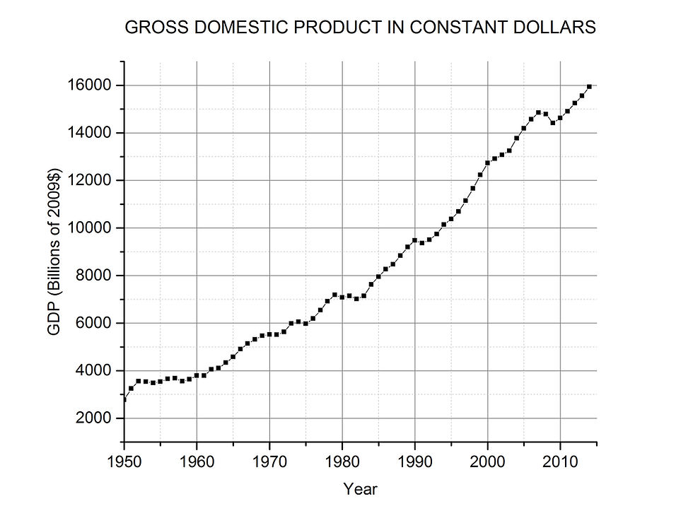
FIGURE 7
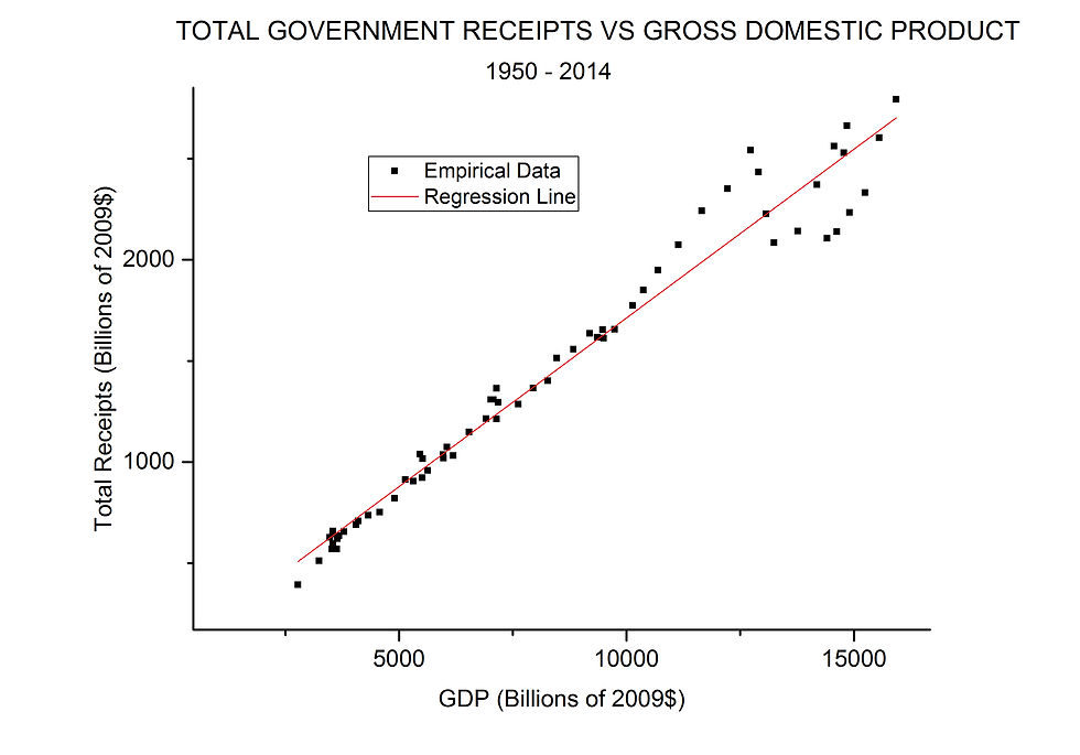
The ratio, receipts/GDP, has a mean value of 0.172 and a standard deviation of .0114 over the years 1950 – 2014. The standard deviation is important because the distribution of sample values of the ratio satisfies both the Shapiro-Wilk and Kolmogorov-Smirnov normality tests. That means that we are justified in thinking of the ratio as a random variable which is normally distributed. For such a distribution there is a 95% probability that any sample value is within 2 standard deviations of the mean. In our case, 95% of the time the ratio should be between 14.9% and 19.5%.
These results mean that the surest way to increase government revenue is not to fool with the tax code in any way, but rather to increase GDP somehow. However I have previously shown through multiple linear regression that the personal income tax rate, corporate income tax rate, capital gains tax rate all together along with population growth rate can only account for about 9.5% of the variation in GDP growth rate. Furthermore, the empirical data show that the GDP growth rate is better when all four of the independent variables increase.
Laffer and Voodoo Revisited
We have seen that the effect of GDP on revenue can be eliminated by expressing all receipts not in any dollars, but rather as a fraction of GDP. With that caveat in mind we can take another look at the evidence that seemed to support “voodoo economics” and the Laffer curve. Figure 8 shows the revision of Figure 2.
FIGURE 8
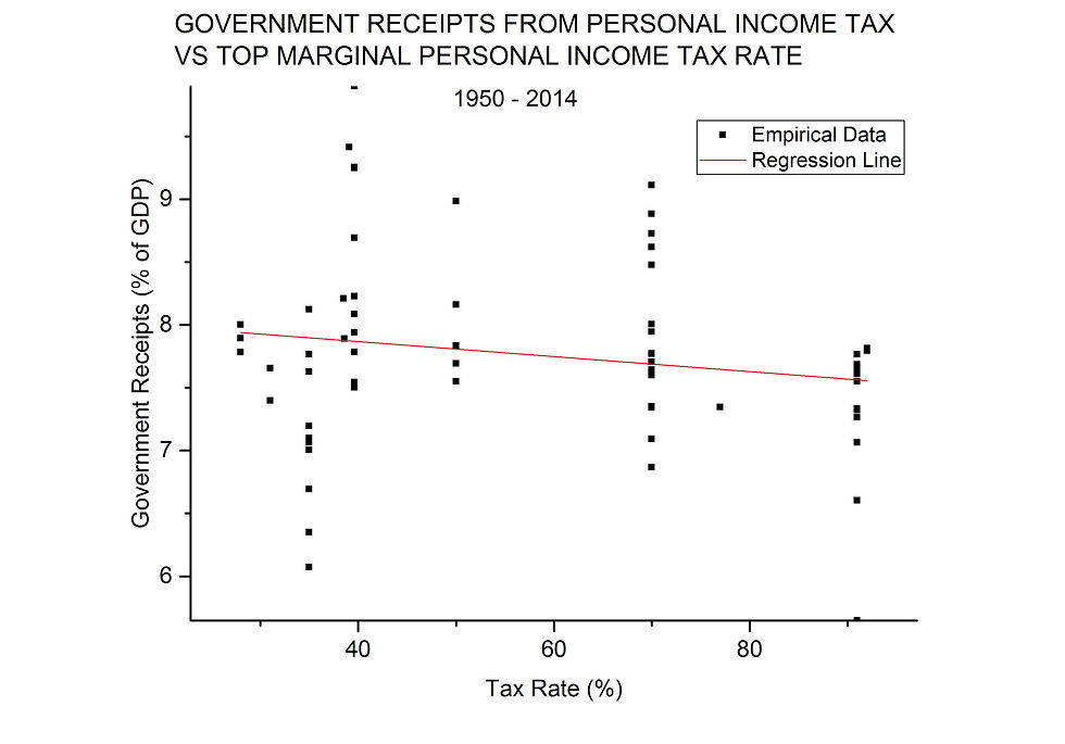
Now the slope of the line is not significantly different from zero (a value meaning no dependence on tax rate), and COD = 0.031. So only about 3% of the variation in receipts could have been due to the tax rate, at least in a linear relationship.
However, several of the peak functions fit the data better than a straight line. The best one is called "Extreme" in Origin and is shown in Figure 9. Once again the fitting equation is available upon request.
FIGURE 9
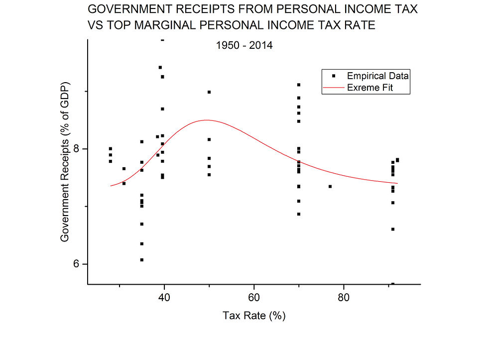
Although the fit is not visually impressive, and the function does not go to zero at the tax rate extremes, it does account for more of the variation seen for historical values of the two variables. What it does not do is provide any succor to those who want to lower personal income tax rates, because the peak in government receipts comes around a tax rate of 50%, well above present levels. Also about 83% of the variation in government receipts from personal income tax is not accounted for by this function.
Next we revisit corporate income tax. The linear regression analysis produces a COD = 0.54 and the plot of Figure 10.
FIGURE 10
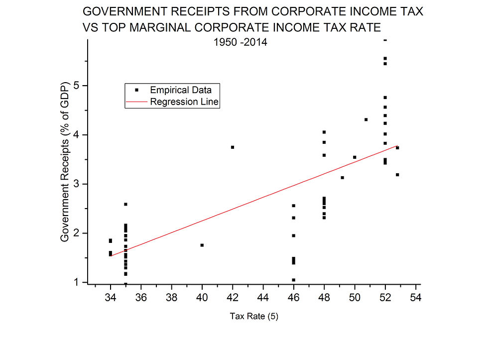
Figure 10 tells a completely different story than Figure 4. Now the slope is significantly different from zero, but positive, indicating more, not less, revenue with increasing corporate tax.
As for peak curves, about eight of them fit the data better (larger COD) than a straight line. All have COD values around 0.75, and they all show peaks at nearly the same place. I only show the “Extreme” function because I used it above above.
FIGURE 11
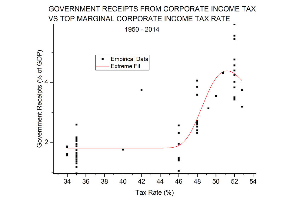
As with personal income tax, this peak fitting function does not indicate that more revenue could be generated by corporate income tax if the tax rate were lowered from its present 35%; the peak appears around 51%, near the highest rate for the whole period.
Why did the data of the earlier section appear to confirm “voodoo economics”? It is because tax rates were generally going down in the period[4] while government receipts and GDP were both going up (see Figures 5, 6, and 12). Without considering GDP, it seemed that the decreasing taxes were causing revenue growth. Once GDP is taken into account, we could see that it was the increase in that variable was the causative factor and lower tax rates were either doing nothing or tending to lower revenue. These results are a cautionary tale about assuming causation, even in the case of high correlation. Even with a COD of 97%, it is not absolutely certain that GDP growth is the cause of revenue growth, although as I said before it is difficult to see how that could not be true and I don’t know of any economist who disagrees.
FIGURE 12
4. Tax Rates and Total Revenue
Once the value of GDP is taken into account, there is only about 3% of the variation in government receipts left to explain. We can only expect to move the ratio receipts/GDP by a couple of percentage points by any tax rate changes. However we should not sniff at a 2 percentage point movement: the budget deficit in 2014 was 2.8% of GDP[5]. Receipts of 19.5% of GDP instead of 17.5% (the actual 2014 value) would certainly have helped. Can lowering any tax rate help in this regard, pushing receipts/GDP higher?
History says not. When we perform linear regression between receipts/GDP and any one of the three top marginal tax rates of Figure 12, the slope of the regression line obtained is not significantly different from zero. The largest COD values is 0.050 for the capital gains tax. Basically, these values indicate that the tax rates have had no statistically significant effect on government receipts measured as a percent of GDP. Furthermore, only personal income tax shows a (statistically insignificant) negative slope.
As a final measure, I tried all three tax rates together in multiple linear regression against receipts/GDP. Then COD = 0.091 or 9.1%: not much of the variation in receipts/GDP can be attributed to all three tax rates together. Only the personal income tax has a negative coefficient, which indicates that a decrease in that rate could increase revenue, but that coefficient is the smallest in magnitude and therefore has the least influence.
Conclusions
1. Hauser’s Law is valid over the period. Total government revenue is proportional to GDP, and that fact accounts for 97% of the variation in revenue. We should expect receipts to be between 14.9% and 19.5% of GDP 95% of the time.
2. For both personal and corporate income tax historical rates, there is some evidence of a single peak curve, if not exactly a Laffer Curve, describing the relation between the tax rate and the revenue collected from that tax. The evidence resides in the fact that the peak curves have higher COD values than straight lines. Both such peak functions have a maximum around a 50% tax rate.
3. There is little empirical support for “voodoo economics” in which reducing any of the present tax rates would increase total government revenue. There is a hint that reducing the top, marginal, personal income tax rate might increase total receipts/GDP, but stronger evidence that such a reduction would decrease GDP. There is also stronger evidence that reducing either corporate income or capital gains top marginal rates would reduce both GDP and total receipts/GDP. Because of the low COD values, it is quite possible that the three tax rates have had no effect on either GDP or receipts/GDP.
Gary Waldman
December 2015
[1] www.whitehouse.gov/omb/budget/historicals, Table 2.1
[2] Ibid, Table 1.3
[3] Ibid, Table 1.2
[4] Historical tax rates can be found on the Internal Revenue Service website, www.irs.gov, or on the website of The Tax Foundation, www.taxfoundation.org
[5] Ibid
TOTAL TAX RATES AND ECONOMIC GROWTH
Introduction
In 2015 I did a simple correlation analysis between the top marginal, federal, individual income tax rate and the GDP growth rate over the 65 year period 1950 – 2014[1]. Although conservative politicians and economists were (and still are) certain that higher taxes slow economic growth, that correlation came out positive, not negative as would be expected if they were right.
Not many people actually pay that top marginal rate on their income. In 2016 another body of tax data became available from the Congressional Budget Office: average or effective federal tax rates on all U.S. income of the tax-paying population for the 35 year period 1979 – 2013. Thinking that this data might be a better measure of tax burden, I again did a correlation analysis between the effective tax rate and GDP growth rate. Once again the result was positive instead of negative[2].
Another factor which might affect GDP growth is population growth. When I included population growth in both of the above analyses it did not change the general conclusion. That is, if the population growth rate were held constant, GDP growth increased rather than decreased with increase in tax rates,
Now another large body of data has become available from the economists Emmanuel Saez and Gabriel Zucman in connection with their book, The Triumph of Injustice. The data is for total taxes paid (federal, state, and local) for the immense time period 1913 – 2018[3]. I have used this body of data for another correlation study with GDP herein, as well as extending the first study to 2018.
Top Marginal Individual Income Tax Rate to 2018
It is easy to extend the linear regression and correlation analysis of reference 1 from a final year of 2014 to 2018 because values for both individual income tax rates and GDP growth are readily available. Adding in the last four years of data (2015 – 2018) changes the correlation coefficient from 0.27 down to 0.22. The coefficient of determination changes from 0.075 to 0.049. Because the correlation coefficient and slope of the regression line are still positive, there is still no evidence of higher tax rates slowing economic growth. Figure 1 tells the new story.
FIGURE 1

Some will point out that the top marginal tax rate went down in 2018 and the GDP growth rate went up, thereby concluding that higher taxes on the rich slow the economy. This is nothing more than confirmation bias via data selection. Anyone making such an assertion should be asked why the 68 other years since 1950 don’t count.
I have started all my analyses in 1950 to avoid the economic distortions of the Great Depression and WW II. However, lest I be accused of my own data selection, I can assure the reader that the correlation from 1930 to 2018 (89 years) is still positive; I have checked it.
Total Tax
The data from reference 3 take the story one step further by considering all U.S. taxes, federal, state, and local including sales taxes. The 2015 and 2017 studies only pertained to federal taxes. The total taxes paid by U.S. residents are expressed as a percentage of national income to get the effective tax rate. National income is defined as[4], “All the income that accrues to the residents of a given country in a given year, whatever legal form this income takes.” This is more than is reported on income tax returns[5]. Once again I used the period from 1950 to 2018, a total of 69 years of data. Tax rates calculated in this manner show a general increase up to about 1995 and then a general decrease since. The history of this effective, total tax rate is shown in Figure 2. The changes appear larger than they really are because the vertical scale is expanded to emphasize them. If the zero of the vertical scale were included, the curve would look much flattened; all values are between 24% and 32 %.
FIGURE 2
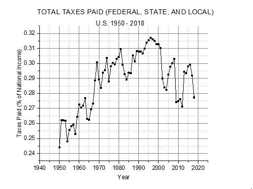
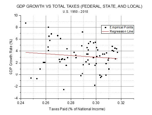
This time a correlation analysis between the tax rate and GDP growth rate does give a negative correlation coefficient and regression line slope. However the magnitude of the correlation (r = -0.12) is far below what is considered statistically significant. The probability that the two variables are unrelated (correlation is really zero) is 16.2%, far above the 5% usually specified for statistical significance. Figure 3 shows the scatterplot and regression line.
It is obvious that the points are widely scattered off the regression line. This scatter leads to coefficient of determination of only 1.5% or, in other words, at least 98.5% of the variation in GDP growth seen over the 69 years must be due to factors other than this total tax rate.
FIGURE 3
If population growth is taken into account along with total taxes in multiple linear regression, the relationship between total tax rate and GDP growth rate becomes positiveagain: GDP growth rate increases with both population growth rate and total tax rate. In this analysis it appears that GDP growth is much more sensitive to population growth than to taxes. The two independent variables taken together can account for only 5% of the variation in GDP growth rate.
I believe that it is fair to say that there is no statistically significant evidence for higher total tax rate slowing GDP growth rate.
Gary Waldman
November 2019
[1] Gary Waldman – Tax Rates and the U.S. Economy (Nov. 2015) – www.garywald.net
[2] Gary Waldman – Higher Federal Taxes Do Not Impede Economic Growth (June 2017) – www.garywald.net
[3] www.taxjusticenow.org. Click on “More” in the upper right of the opening page, and pick “Technical Appendix”. On the ensuing page click on “Supplementary tables underlying statistics presented in the book”. I used column L of Table TA3.
[4] E. Saez & G. Zucman – The Triumph of Injustice – W. W. Norton & Co. (2019), p. 14
[5] Ibid
Comments